Metadynamics

For an up to date list of pubblication on this subject, see this page.

The method is aimed at reconstructing the multidimensional free energy of complex systems, and is based on an artificial dynamics (metadynamics) performed in the space defined by a few collective variables S, which are assumed to provide a coarse-grained description of the system (see Ref. [1] and, for a recent review, Ref. [2]). The dynamics is driven by the free energy and is biased by a history-dependent potential constructed as a sum of Gaussians centered along the trajectory of the collective variables. If a new Gaussian is added at every time interval t_G, the biasing potential at time t is given by

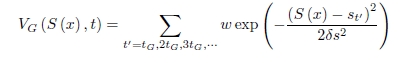
where w and ds are the height and the width of the Gaussians and s_t=S(x(t) is the value of the collective variable at time t. This potential, in time, fills the minima in the free energy surface, i.e. the sum of the Gaussians and of the free energy becomes approximately a constant as a function of the collective variables.

This approach can be exploited not only for efficiently computing the free energy, but also for exploring new reaction pathways and accelerating rare events.

• In the example in figure, the dynamics is started from the minimum at the center. This minimum is quickly filled with Gaussians, and the system evolves through the lowest saddle point, the one at the left. This illustrates how the method has the property of making the system escape local free energy minima through the lowest free energy saddle point.
• Afterwards, the dynamics continues, and all the free energy profile is filled with Gaussians. At the end, the sum of the Gaussians provides the negative image of the free energy. This illustrates how the method can be used for estimating the free energy .

The collective variables

The gist of the method is to identify the variables that are of interest and that are difficult to sample, since the stable minima in the space spanned by these variables are separated by barriers that cannot be cleared in the available simulation time. These variables S(x) are functions of the coordinates of the system, they can be up to three in practical applications, and they depend on the process that one wants to study. For example, in a chemical reaction one can use as collective variables all the coordination number between the atomic species involved in the reaction (see Ref. [2] for more details).


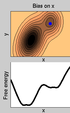Consider the example in figure. The dynamics of the system takes place on a 2-dimensional potential energy surface. The normal dynamics is biased by a metadynamics potential acting on x. Then, in this specific case, S(x)=x. In the lower panel, we show the free energy (thick line), and the sum of the free energy and the history-dependent potential at various simulation times (thin lines).

After a transient, the sum of V_G(s,t) and of F(s) becomes approximately flat, indicating that V_G(s,t)~-F(s). This allows estimating the free energy as the time average of all the V_G(s,t).

In reference [3] it is shown that each V_G(s,t)~-F(s) is an unbiased estimator of the free energy if the dynamics along s is very slow compared to the dynamics along the transvere degrees of freedom (y in the example in Figure). As it is clear from the movie, even if this condition is violated the history-dependent potential estimates reather accurately the free energy.

However, choosing the correct collective variable in applications can be far from trivial. If the

[1] A Laio, M Parrinello,
Escaping free-energy minima
PROCEEDINGS OF THE NATIONAL ACADEMY OF SCIENCES OF THE UNITED STATES OF, 99, 12562 (2002)

[2] A Laio, FL Gervasio,
Metadynamics: a method to simulate rare events and reconstruct the free energy in biophysics, chemistry and material science
REPORTS ON PROGRESS IN PHYSICS, 71, 126601 (2008)

[3] G Bussi, A Laio, M Parrinello,
Equilibrium free energies from nonequilibrium metadynamics
PHYSICAL REVIEW LETTERS, 96, 090601 (2006)